• Preface
• Introduction
• The program
• Description of the input parameters
• Description of the output
• Example

Preface

Introduction

• at every point on the grid is exp(-E/kT) where E is the interaction energy at the point, k - Boltzmann constant, T - temperature.
• The average Boltzmann factor within a reaction distance is computed as an average over all points not leading to overlaps and satisfying the reaction conditions within the specified distance. This allows to have a factor that is already scaled by average Boltzmann factor with no interactions.
• The orientation averaged Boltmann factor on the grid is computed as an average over all random orientations of the protein, while its center is kept fixed.

• sdabf computes the average Boltzmann factor within the reaction distance which gives the estimate for rate enhancement due to interactions. The reactions may be defined exactly as in sda. It is necessary to have the UHBD computed electrostatic potential (of only the first protein) and ecm generated charges of the second protein in hand.
• sdabf also computes 2 grids, one with the orientation-averaged Boltzmann factor at each point and the other with the Boltzmann averaged electrostatic interaction free energy value at each point of the grid.  Sampling and averaging is carried out as follows: one protein is kept fixed and the center of the other protein is placed at grid points and its orientations are sampled randomly.

• The estimates will not be accurate if the reaction patch is large, although qualitatively the results are found to follow the trends revealed by Brownian dynamics simulations.
• The average Boltzmann factor provides only a rough approximation of the rates computed by the sda Brownian dynamics program

The program

Description of the input parameters

The description of each number follows:

dseed - random number generator seed. Defines the sequence of random numbers used to model the Brownian dynamics. Different numbers result in different sampling and trajectories.

nrun - the number of random angles at every point of the sampling grid to be tried to compute the average Boltzmann factor.

probes, thres, hexcl, dsfactor - the probe radius used to represent the second protein atoms and the threshold value for atomic accessibility. The atoms of protein 2 having accessibilities less than thres are not used in computing exclusion. hexcl is the spacing for the exclusion grid of protein 1.  dsfactor is a factor to multiply the desolvation penalty grid (see the description of the desolvation term).

pdb1f, pdb2f - the names of files with atomic coordinates of proteins 1 and 2, in pdb format ('ATOM',a24,3f8.3).  The first protein file may have a record giving the scaling factor for its radius, after the coordinate record: ('ATOM',24x,3f8.3,f15.8) when the sdabfsc program is used.  If no record is present, then the factor is 1.0.

po1f - the name of the file with the electrostatic potential of protein 1. UHBD binary format. po2f - not used here, but it is read in.

qef2f - the names of files with charges for proteins 1 and 2. ('ATOM',24x,3f8.3,f15.8). qef1f - not used here, but it is read in.

rxna1f, rxna2f - the names of files with reaction atom coordinates for proteins 1 and 2 in pdb format. ('ATOM',24x,3f8.3).

ic1fix, xc1 - 2 lines, the integer on the first line is 1 or 0, the second line defines the coordinates of the center of the first protein supplied by the user. These coordinates used by the program when ic1fix=1, and recomputed when ic1fix=0.

ic2fix, xc2 - the same as above for the second protein center.

icomm - switches the encounter complex modeling options. icomm=1-3 deal with 3 different ways to count reaction events: icomm=1 counts RMSD reaction conditions icomm=2 interresidue contact pairs, icomm=3counts independent contact pairs among all possible donor-acceptor pairs formed between the 2 proteins. Refer to readme for Brownian dymnamics program.

iforce =0 switches off all the interaction forces except the exclusion forces. iforce =1 is the standard option when the forces are computed using the potential grid of protein 1 (2) and the charges of protein 2 (1). iforce =2 does not use the potential grids at all but computes the forces using the charges alone - this is efficient only when the number of charges is less than 10. Charge-charge treatment is useful when a large executable is not affordable as a separately compiled small executable can be used. For iforce =2, it is necessary to give the correct value of aiostr == ionic strength of the solvent in mM.

dm, dr, drI , irot2f - not used here.

b, c - not used here.

rboost, novers not used here.

dt1, swd1, dt2, swd2, rswd - not used here.

win0, dwin, nwin - the reaction complex will be recorded for each of nwin contacts (or RMSD distances) d_i, i=1,nwin. d_i=win0+(i-1)*dwin. If iwrec.ne.0 then the positions of the second protein will be written to file fort.55, when 2 contacts at distance d_nwrec are satisfied.
dspo1f, dspo2f - the names of files with charge desolvation penalties of proteins 1 and 2. UHBD binary format.  dspo2f - is not used, but read in.Charge desolvation free energies computed by a separate program in sda distribution mk_ds_grd.f.  See description of charge desolvation in sda.html.
igwrite - Option to write grids or not: igwrite=1 - the program will calculate and write grids, iform=0 - only the table of Boltzmann factors as a function of contact distance is written.

hs,nsx,nsy,nsz - the parameters of the sampling grid: the program will make nrun samplings of random angles at every point of the grid, compute reaction conditions and add up the Boltzmann factors if the conditions are satisfied, thus creating the table of Boltzmann factors at every reaction distance.  hs - spacing of the sampling grid, nsx,nsy,nsz - its dimensions. It is centered at the center of the second protein, given in pdf2f.  It has to be large enough that all important interaction regions are included (to get the complete sampling for the Boltzmann factor grids as well as to have correct Boltzmann factors at each reaction distance).
psof,psofe,iform -  The names of the grids to write the orientational Boltzmann factor average and Boltzmann averaged electrostatic interaction energy and their format (iform=1 - ascii, iform=0 - binary UHBD format).

The output files

The file fort.66 contains the length of each trajectory.

The file fort.77 contains the electrostatic potentials of protein 1 and protein 2 along 5 selected lines in 3-dimensional space; a section through the exclusion grid in ascii format in the plane passing through the center of protein 1; reaction atom information.

Since the above files are overwritten each program run, one needs to rename them after the execution if they are needed.

The file runs.done has the number of runs (orientational samplings) performed so far. The information is written every 50 runs and is useful when the printout frequency is low and the machine writes to files with buffering.

Standard output (fort.6) has the following.

• number of samplings = nrun*nsx*nsy*nsz;
• number of overlaps (when the step is repeated) occurred.

---

Example

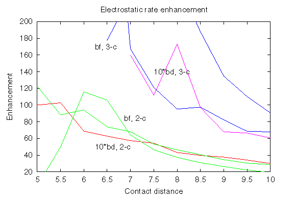
Here the rate enhancements are shown, which were obtained by computing Boltzmann factors (marked bf) for the encounter complexes defined by  2 or 3 contacts at the distance specified on the x-axis; there are 2 curves for each Boltzmann factor, which correspond to 2 different ways of sampling the Boltzmann factors. The rate enhancements obtained by BD simulations are marked bd, and by the number of contacts, 2 or 3. In fact, the BD rate enhancements are multiplied by 10 to bring the 2 estimates into quantitative correspondence. Consequently, the ratio of rate enhancements for encounter complexes defined by 2 and 3 contacts is reproduced reasonably well by sampling of the Boltzmann factor. The Boltzmann factor overestimates by a factor of 10 the rate enhancement obtained by BD. Partially, this overestimation is due to applying a cutoff to the interactions at a 54 Å distance of (Protein I centre)-(Protein II charge). The sampling of the Boltzmann factor is insensitive to this cutoff. On the other hand, BD simulations are sensitive to this cutoff, although,  this cutoff contribution to rate enhancement has been shown not exceed a factor of 2.

Acknowledgements

Viel Spass. 

Rebecca Wade

February 2000